If you are relying on built-in functions to read and write large datasets you are losing out on efficiency and speed gains available through external packages in R. Below, I benchmark some of the options out there used for reading and writing files.
Sample Data
First, I’ll generate a sample dataset with ten million rows we can use for testing.
Generating a test dataset
library(tidyverse)
library(microbenchmark)
n <- 1e6
times <- 10 # Number of times to run each benchmark
data <- data.frame(a = runif(n),
                   b = sample(1:1000, n, T),
                   c = sample(month.name, n, T),
                   d = sample(LETTERS, n, T))

write.table(data, "data.tsv", quote = F, row.names = F)
Here are the first few rows of that dataset:
| a | b | c | d | |
|---|---|---|---|---|
| 1 | 0.1926477 | 789 | August | R |
| 2 | 0.8303095 | 156 | March | D |
| 3 | 0.1144189 | 742 | July | P |
| 4 | 0.2828960 | 337 | April | S |
| 5 | 0.2861664 | 43 | November | W |
Reading TSVs
Base R has some pretty slow functions for reading files that also are poorly designed (row numbers and quotes by default, issues reading column names with special characters, etc.). Lets see how they compare with more up to date packages.
vroom vs readr vs base R vs data.table
Below I use microbenchmark to compare the following methods for reading this 1M row dataset:
base::read.tablebase::read.delimreadr::read_tsvvroom::vroomdata.table::freadtbl_df(data.table::fread)- This converts the data.table to atibble::tbl_dfobject which is the type of data structurereadrandvroomreturn and is what is used in the tidyverse.
These functions will output data in either a data.frame, tibble, or data.table.
bm <- microbenchmark(
  `base::read.table` = read.table("data.tsv"),
  `base::read.delim` = read.delim("data.tsv"),
  `readr::read_tsv` = readr::read_tsv("data.tsv"),
  `vroom ~ 1 thread` = vroom::vroom("data.tsv", num_threads = 1),
  `vroom ~ 8 threads` = vroom::vroom("data.tsv"),
  `tbl_df(data.table::fread) ~ 1 thread` = tbl_df(data.table::fread("data.tsv", nThread = 1)),
  `tbl_df(data.table::fread) ~ 8 threads` = tbl_df(data.table::fread("data.tsv")),
  `data.table::fread ~ 1 thread` = data.table::fread("data.tsv", nThread = 1),
  `data.table::fread ~ 8 threads` = data.table::fread("data.tsv"),
  times = times
)
autoplot(bm) +
  labs(caption = glue::glue("{scales::comma(n)} rows; {times} times"))
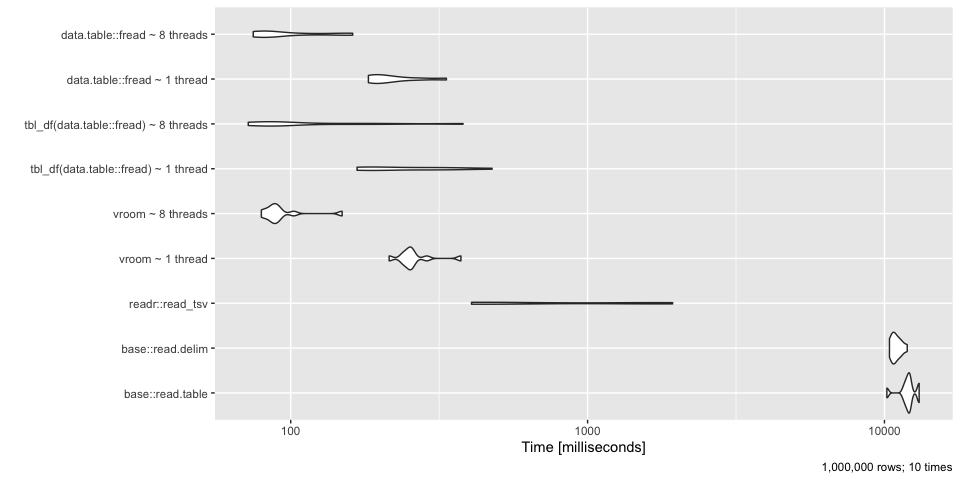
Looks like the base R functions lose - by a lot. data.table::fread and vroom::vroom come out on top at ~ 100 milleseconds whereas the base functions take ~10 seconds or 100x longer!
Stop wasting your time with read.table, read.csv, and read.delim and move to something quicker like data.table::fread, or vroom::vroom both of which perform much faster. Both can also take advantage of multiple cores but outperform base R even when they only use a single thread!
Writing TSVs
vroom vs readr vs data.table vs base R
Next I compared methods for writing TSV files. Base R has the functions write.csv and write.table for writing delimited text files. Unfortunately, these too have poor defaults (quoting strings, adding rownames). I have turned these off for the comparison.
bm <- microbenchmark(
    `base::write.table` = write.table(data, file = "out.tsv", quote=F, sep = "\t"),
    `readr::write_tsv` = readr::write_tsv(data, "out.tsv"),
    `readr::write_tsv + gz` = readr::write_tsv(data, "out.tsv.gz"),
    `data.table::fwrite ~ 1 thread` = data.table::fwrite(data, "out.tsv", nThread = 1),
    `data.table::fwrite ~ 8 threads` = data.table::fwrite(data, "out.tsv", nThread = 8),
    `vroom::vroom_write ~ 1 thread` = vroom::vroom_write(data, "out.tsv", num_threads = 1),
    `vroom::vroom_write ~ 8 threads` = vroom::vroom_write(data, "out.tsv"),
    `vroom::vroom_write ~ 1 thread + gz` = vroom::vroom_write(data, "out.tsv.gz", num_threads = 1),
    `vroom::vroom_write ~ 8 threads + gz` = vroom::vroom_write(data, "out.tsv.gz"),
    times = times
)
autoplot(bm)
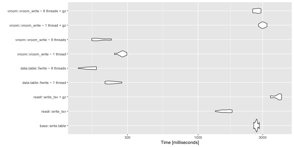
data.table::fwrite performs the fastest in multi-threaded mode with vroom::vroom not far behind. These are ~100x faster than base R. Apparently, applying gzip compression slows things down considerably but can save a lot of space.
Serializing Data
Serialized data formats retain column types and avoid data loss that may occur when writing and reading TSVs. Here I compare:
feather::write_featherfst::write_fstbase::savebase::saveRDS
Note that these serialization formats each provide other benefits that should be considered. For example, feather files are a good interchange format between R and python using the python Pandas module.
bm <- microbenchmark(
   `base::save`=save(data, file = "out.Rda"),
   `saveRDS` = saveRDS(data, file = "out.rds"),
   `fst::write_fst` = fst::write_fst(data, path = "out.fst"),
   `feather::write_feather` = feather::write_feather(data, path = "out.feather"),
   times = times
)
autoplot(bm)
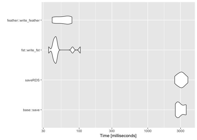
fst and feather perform about the same and again, about ~100x better than base R.
Reading Serialized Data
bm <- microbenchmark(
   `base::load`=load(file = "out.Rda"),
   `readRDS` = readRDS(file = "out.rds"),
   `fst::read_fst` = fst::read_fst(path = "out.fst"),
   `feather::read_feather` = feather::read_feather(path = "out.feather"),
   times = times
)
autoplot(bm)
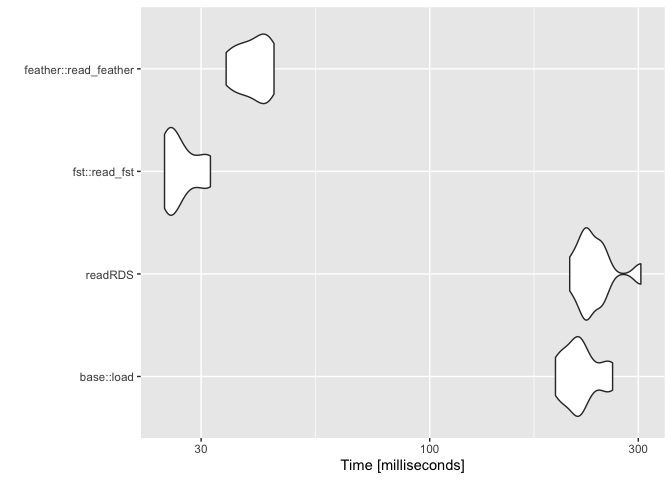
fst reads the quickest but feather is not too far behind. These functions are about ~10x better than base R in this comparison.